SatSim: from satellite imagery to observations

SatSim represents a scene as a georeferenced satellite GeoTIFF. Given a pose and camera settings, it computes ground coverage, reads local imagery, rotates by heading, and resizes to the model’s RGB input. The camera uses a downward-looking model over a ground plane; altitude controls observation scale.

1. Connecting geographic positions to pixels

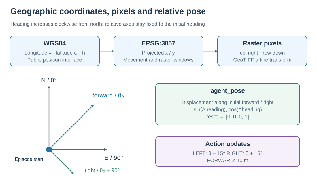
The relative forward/right axes are set by the initial heading and stay fixed throughout the episode. Action magnitudes in the figure use standard settings.

Representation	Units and directions	Role
WGS84 [longitude, latitude, altitude]	Longitude/latitude in degrees, altitude in meters	Episodes and public agent state
EPSG:3857 (x, y)	Web Mercator projected meters; x east, y north	Internal position and raster windows
GeoTIFF (row, col)	Rows downward, columns rightward	Raster pixel access
Initial-heading (forward, right)	Ground meters relative to episode start	Displacement in agent_pose

The GeoTIFF coordinate reference system and affine transform connect projected coordinates to pixels. SatSim opens scenes in EPSG:3857 and reuses open datasets for repeated access to a scene.

The local Web Mercator scale factor at latitude \(\varphi\) is \(k=1/\cos\varphi\). Rendering multiplies ground coverage by \(k\) to obtain projected window dimensions; movement uses the same local conversion. Configured forward distances and camera coverage are therefore expressed in ground meters.

2. Altitude, field of view, and coverage

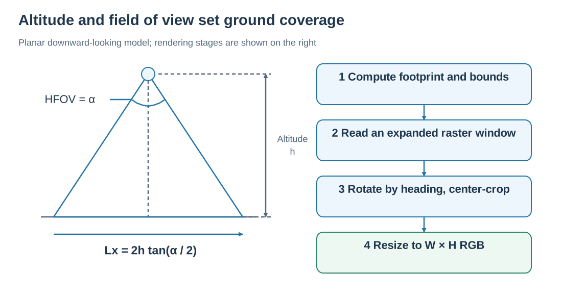
Left: the horizontal field-of-view cross section. Right: the rendering sequence.

For altitude \(h\), horizontal field of view \(\alpha\), and output dimensions \(W,H\), the unrotated footprint over the ground plane has dimensions:

\[ L_x=2h\tan(\alpha/2),\qquad L_y=L_x\frac{H}{W}. \]

With 448 × 448 output and 90° HFOV, altitude 50 m gives approximately 100 × 100 m coverage. At 100 m altitude, coverage grows to approximately 200 × 200 m, so the same building occupies fewer output pixels. Increasing HFOV at fixed altitude also expands coverage.

Output resolution sets how many pixels represent this region; the source GeoTIFF resolution determines the imagery detail available to sample.

3. Camera comparisons on a real scene

The figures below use one fixed center in Amsterdam-1.tif. All RGB observations come from the current SatelliteCamera.render_image() with 448 × 448 output. Colored outlines in the context map show footprints; the other panels show their rendered observations.

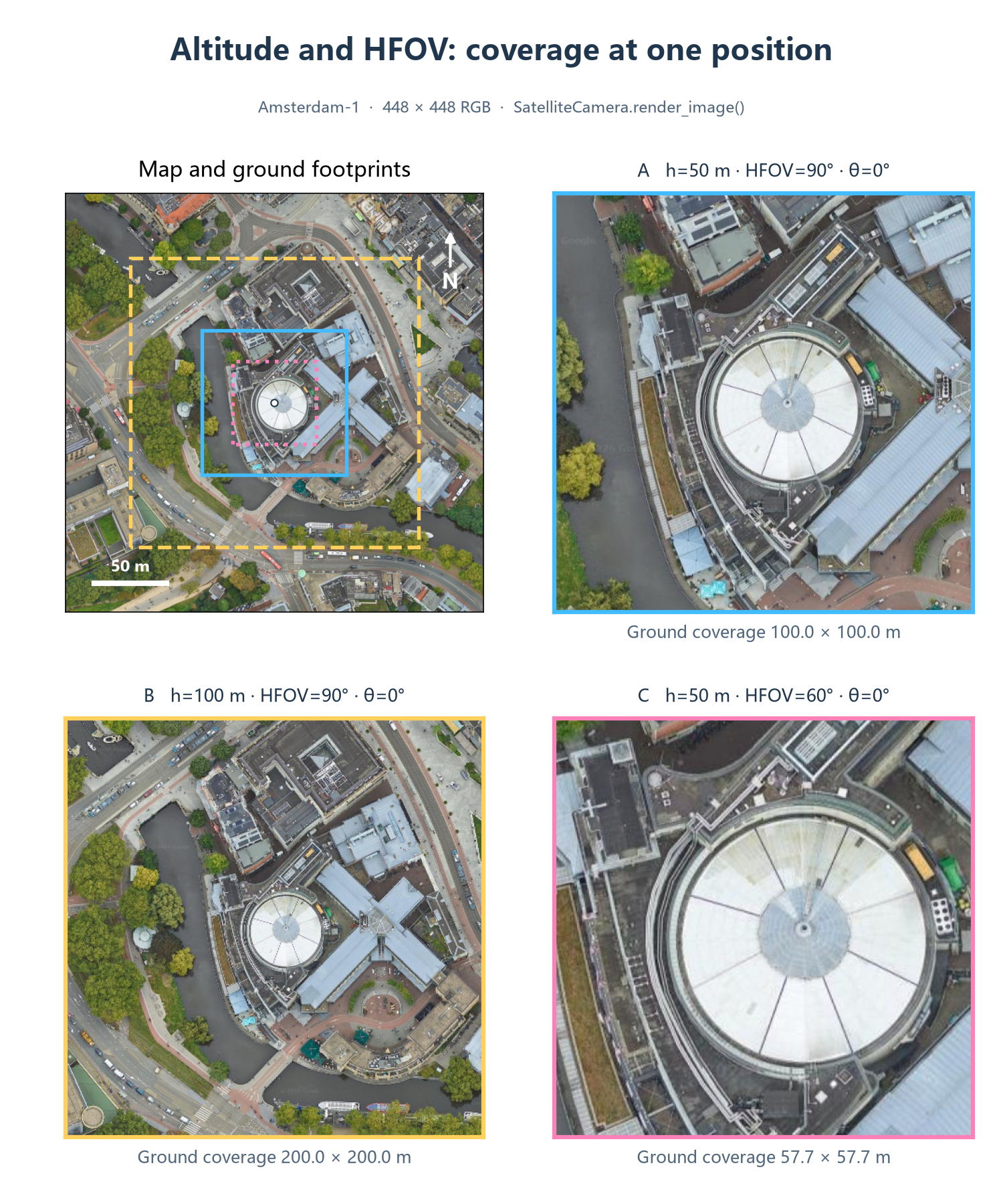
A: h=50 m, HFOV=90°; B: h=100 m, HFOV=90°; C: h=50 m, HFOV=60°. Heading is 0° throughout. Coverage widths are approximately 100 m, 200 m, and 57.7 m.

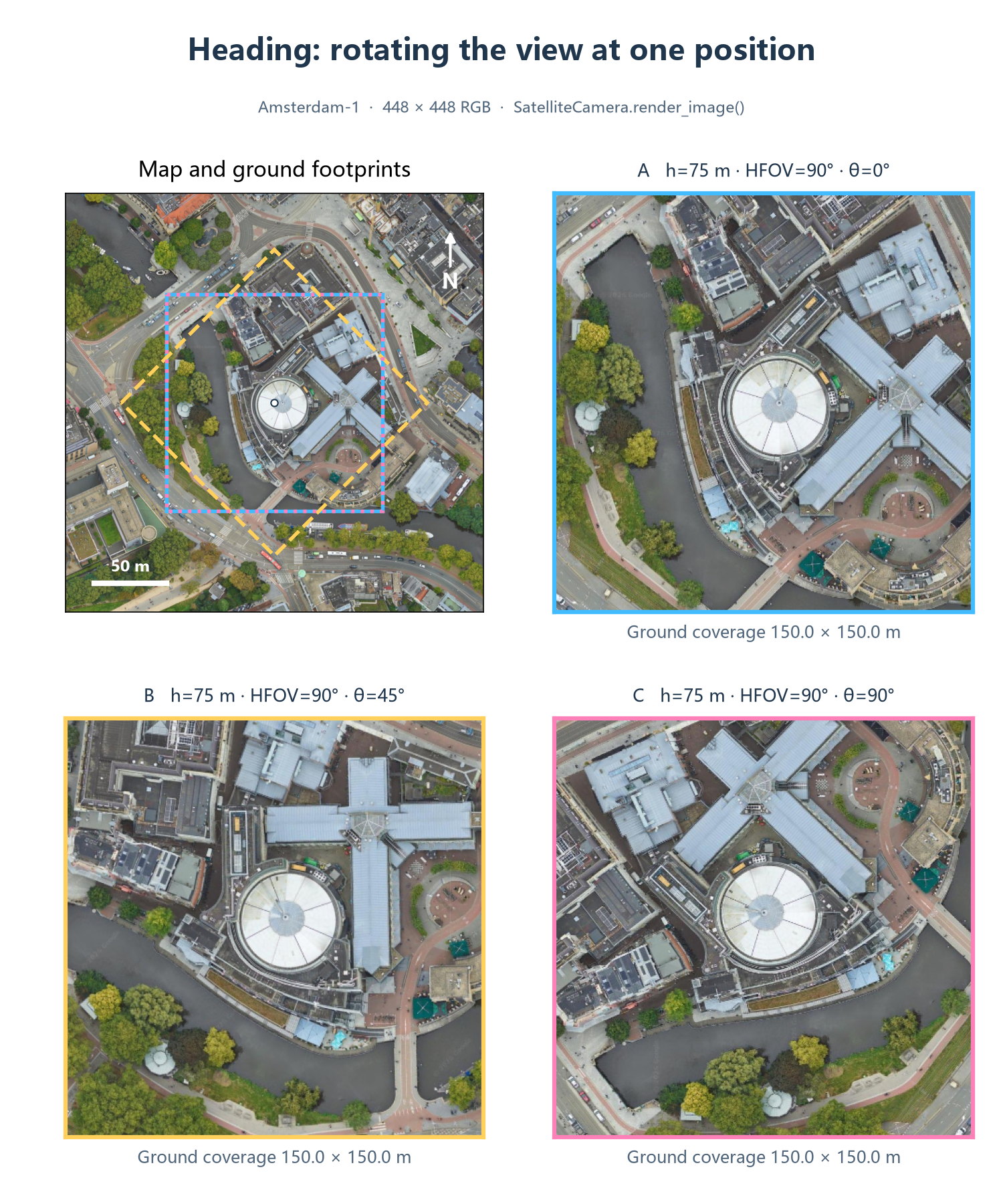
At h=75 m and HFOV=90°, compare heading 0°, 45°, and 90°. Changing heading rotates the footprint and the rendered image content.

4. Rendering RGB

SatelliteCamera.render_image() performs four stages:

1. Compute the footprint from altitude, HFOV, aspect ratio, and latitude scale; rotate its corners and obtain an axis-aligned bounding box.

2. Check the rotated extent against scene bounds and read an expanded window covering the rotation.

3. Rotate that window with OpenCV using heading, then center-crop to the requested coverage dimensions.

4. Resize to configured WIDTH × HEIGHT, returning (H, W, 3) uint8 RGB.

A square footprint covers the same square at 0° and 90°, while the output orientation changes. At 45°, its axis-aligned bounding box is larger. Outlines in the figures show rotated quadrilaterals; raster reads use their bounding extent.

5. Updating position and heading

Heading \(\theta\) increases clockwise from north: 0° is north and 90° is east. A forward action with ground distance \(d\) uses the local scale \(k\):

\[ x'=x+kd\sin\theta,\qquad y'=y+kd\cos\theta. \]

Standard settings use \(d=10\) m and turn angle \(\beta=15°\). Left turns update to \(\theta-\beta\), right turns to \(\theta+\beta\), normalized to \([0°,360°)\). All four primitive actions preserve altitude.

Boundary handling has two stages. is_navigable() computes an inset map region using altitude and camera aspect ratio to accept or reject a candidate position. Rendering then checks the actual rotated window. A rejected forward move leaves the agent in place and still consumes a step. A rendering window outside the raster raises an error; the Viewer or evaluation record helps locate that state.

6. Interpreting relative pose

agent_pose returns:

[delta_forward_m, delta_right_m, sin(delta_heading), cos(delta_heading)]

Displacement is measured from the start along the initial-heading forward/right axes. The implementation first estimates east/north displacements \(\Delta E,\Delta N\) from longitude/latitude differences using a local spherical approximation at the midpoint latitude. It then rotates by initial heading \(\theta_0\):

\[ \Delta f=\Delta N\cos\theta_0+\Delta E\sin\theta_0,\qquad \Delta r=\Delta E\cos\theta_0-\Delta N\sin\theta_0. \]

Starting east and moving 10 m east gives approximately forward=10 m, right=0 m. Turning right by 90° in place preserves those displacement components and changes the heading encoding to approximately [1, 0]. The sin/cos encoding keeps nearby headings close across angle wraparound.

Implementation: SatelliteCamera, SatSim, GeoUtils, AgentPoseSensor, and lonlat_to_ego_displacement. See the Viewer for visualization and Core API for parameters.