Historical memory: sampling, per-frame compression, and token clustering

简体中文 | English

Historical memory turns observations before the current window into a compact feature sequence. Its variants change which images are read, how visual tokens are combined, and which temporal and spatial relationships the output preserves. See dual memory and sliding windows for update timing and memory configuration for launch commands.

1. Inputs and outputs

The counts below use the Qwen2.5-VL image grid produced by the code for 448 × 448 inputs: each frame has \(16\times16=256\) tokens after the vision encoder and its native spatial merge.

Mechanism	Historical input	Output organization	Typical budget
Short-term only	No pre-window images	Window dialogue only	0
Per-frame pooling	Up to 8 sampled frames	Pool each frame spatially; concatenate chronologically	\(8\times64=512\)
GridToMe	Up to 8 sampled frames	Aggregate within spatial regions; concatenate by frame	512 on the reference grid
GTC	All pre-window query frames	Cluster all frames jointly	At most 512
STC / Segment-GTC	All pre-window query frames	Cluster within 8 temporal segments; concatenate segments	At most 512

NUM_HISTORY controls per-frame sampling. GTC/STC training reads frames at 0,k,2k,…<b, where \(k\) is the action-prediction interval and \(b\) the window start. Evaluation uses cached features from actual queries before the boundary. Per-frame sampling instead draws from RGB observations at every pre-window action step.

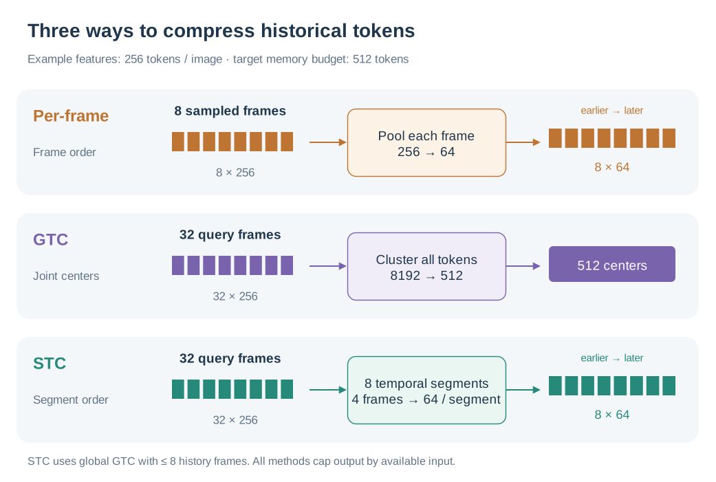
Blocks illustrate image or token groups; the labels give the actual token budgets.

2. Selecting historical frames

For a prefix of \(H\) frames, select at most \(n=\min(n_{\mathrm{req}},H)\) frames, where \(n_{\mathrm{req}}\) is NUM_HISTORY. Deterministic sampling starts with \(u_i=i/(n-1)\) and maps it to:

\[ q_i=1-(1-u_i)^b,\qquad r_i=\operatorname{round}\big(q_i(H-1)\big). \]

The exponent \(b\) is called LOG_BASE in the code. \(b=1\) covers history uniformly; \(b=2\) puts more samples near the recent end. For \(H=100,n=5\), uniform sampling gives approximately [0,25,50,74,99]; temporal bias gives [0,43,74,93,99].

Random sampling selects uniformly without replacement, then sorts the indices chronologically. Deterministic sampling fills rounding collisions with the earliest unused frames. A single requested frame selects the most recent one; when fewer frames are available than requested, all are used. Training and evaluation share sample_per_frame_history_indices().

3. Per-frame: compress each image, then concatenate

Let \(X_i\in\mathbb R^{h\times w\times d}\) be one frame’s visual features. Average pooling with stride \(s\) averages each local \(s\times s\) region:

\[ \bar X_i[a,b]=\frac{1}{s^2} \sum_{u=0}^{s-1}\sum_{v=0}^{s-1}X_i[sa+u,sb+v]. \]

The implementation restores the spatial grid, calls avg_pool2d(kernel_size=s, stride=s), then flattens it. The output has \(\lfloor h/s\rfloor\lfloor w/s\rfloor\) tokens. With \(h=w=16,s=2\), each frame contributes 64 tokens; eight frames form a 512-token block in chronological order.

This preserves frame order and each frame’s downsampled spatial layout. Similar buildings in adjacent views can still occupy separate tokens because compression is independent across frames.

How GridToMe replaces pooling

USE_TOME=true selects the repository’s grid aggregation implementation. Each frame is divided into \(2\times2\) regions. Adaptive average pooling initializes centers within each region, followed by cosine-similarity aggregation. For region tokens \(x_i\) and centers \(c_j\):

\[ w_{ij}=\frac{\exp(\cos(x_i,c_j)/0.1)} {\sum_{i'}\exp(\cos(x_{i'},c_j)/0.1)},\qquad z_j=\sum_i w_{ij}x_i. \]

Each center normalizes weights over input tokens, implemented as softmax(sim, dim=0). On the reference grid, each region reduces \(8\times8\) tokens to \(4\times4\), giving 64 tokens across four regions. Outputs are concatenated by region and then by frame time. Small regions trigger a fallback to ordinary pooling.

4. GTC: soft k-means across frames

GTC concatenates historical features into \(X\in\mathbb R^{M\times d}\) and uses \(K=\min(K_{\max},M)\) centers, where \(K_{\max}\) is GTC_OUTPUT_TOKENS. By default, centers are initialized from uniformly spaced tokens in this sequence, the temperature is \(\tau=0.1\), and one update is performed.

Each token first receives a soft assignment over centers:

\[ A_{ij}=\frac{\exp(\cos(x_i,c_j)/\tau)} {\sum_{j'}\exp(\cos(x_i,c_{j'})/\tau)}. \]

Centers are then updated by weighted averaging:

\[ c'_j=\frac{\sum_i A_{ij}x_i}{\sum_i A_{ij}}. \]

Cosine similarity uses normalized vectors; the update aggregates the original feature values. Assignments normalize along the center dimension with softmax(..., dim=-1), followed by division by each center’s total assigned weight. This differs from the GridToMe weighting above.

For example, 32 historical query frames produce \(32\times256=8192\) input tokens that GTC aggregates into 512. Similar tokens from different times can contribute to the same center. Outputs have no explicit per-frame grouping; temporal information can remain indirectly in the features and initialization. If the input already fits the target budget, the implementation returns it directly.

Clustering introduces no learned centroid parameters. Centers are initialized from the current historical features. Softmax and weighted aggregation remain in the training computation graph, allowing gradients to reach the vision encoder and input enhancement modules.

5. STC: GTC within temporal segments

STC is implemented as SegmentGTC, selected by segment_gtc. With more than eight history frames, it divides the sequence into eight contiguous segments of approximately equal frame count. Each segment runs GTC independently, and outputs are concatenated from early to late:

\[ L=[\operatorname{GTC}(X^{(0)});\ldots;\operatorname{GTC}(X^{(7)})]. \]

With 32 frames and a 512-token budget, each segment contains four frames, or 1024 input tokens, and outputs 64. Centers in later segments aggregate only later observations, preserving a coarse temporal structure.

The implementation also specifies these boundary cases:

• Remainder frames are assigned to earlier segments; remainder output tokens are assigned to later segments.

• With at most eight history frames, it performs global GTC instead. Inputs that fit the budget are returned as a concatenated sequence.

• Each segment outputs at most its available token count. Unused capacity stays with that segment, so the general output count is the sum of min(segment budget, segment input count).

6. Token budget and computation

At the same output budget, per-frame sampling limits how many images must be encoded, while GTC/STC retain more historical input before compression. For \(M\) input tokens, \(K\) centers, and feature dimension \(d\), one GTC similarity computation costs approximately \(O(MKd)\) and creates an \(M\times K\) assignment matrix. STC processes segments separately, reducing the size of each individual matrix.

Examples using the reference visual grid:

Window start and setting	Historical input	Memory output
Start 0, ordinary history memory	0 frames	0
Start 32, per-frame, 8 frames, stride 2	\(8\times256\)	512
Start 32, GTC, action interval 4	\(8\times256\)	512
Start 128, GTC, action interval 4	\(32\times256\)	512
Start 128, STC, action interval 4	8 segments of \(4\times256\)	\(8\times64=512\)

For other image sizes or visual backbones, compute token counts from the actual image_grid_thw and merge_size. The 512-token budget here covers long-term memory; total LLM context also includes the instruction, full window images, action text, and optional initial image.

7. Code and paper references

Component	Code
Per-frame sampling and chronological concatenation	per_frame.py
Spatial pooling and GridToMe	compressor.py
Soft k-means and global clustering	gtc.py
Segmentation, budgets, and short histories	segment_gtc.py
Training history source	SwiftVLNDataset._sample_history_frames
Evaluation sampling, feature reuse, and clustering	VisualEncodingMixin

Paper source: SatNav paper, Memory Design Details → History Frame Sampling / GTC / STC. The GridToMe computation and STC boundary behavior are documented from the current code.