Map memory: encoding explored space as visual context

简体中文 | English

Map memory represents pre-window spatial experience with two north-up maps. A global map provides large-scale route context; a local map shows detail around the window start. Both pass through the same vision encoder as current observations and populate <history_memory>. They follow the same window-boundary update schedule as other long-term memories.

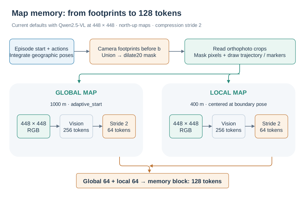
The two maps share the vision encoder, are pooled separately, and are concatenated as historical memory.

1. Turning a trajectory into two maps

Rendering uses the SatNav scene orthophoto, episode start coordinates and heading, executed actions, camera field of view, and altitude:

1. Convert the start to Web Mercator coordinates and integrate forward steps and turns into a pose sequence.

2. For a new window starting at \(b\), use poses with indices below \(b\) to define observed space. The trajectory polyline includes the position at the boundary.

3. Compute each observation’s ground-footprint polygon from altitude, horizontal field of view, aspect ratio, and heading. Combine the footprints into a mask.

4. Read square global and local crops from the orthophoto and set pixels outside the mask to black.

5. Draw the trajectory in red, start in blue, and current position and heading in yellow. Return [global_map, local_map].

For a downward-facing camera, footprint width is \(2h\tan(\mathrm{HFOV}/2)\); image aspect ratio determines footprint height. Geographic conversion includes the latitude-dependent Mercator scale so map side lengths remain ground distances in meters.

The current position in this memory is the new window’s starting position. The map remains that snapshot while actions execute within the window, until the next slide.

2. Global view, local view, and explored mask

Component	Current default	Role
Global map	1000 m side length	Overall route and starting-area relationships
Local map	400 m side length, centered at the window start	Nearby spatial detail
Render resolution	448 × 448 for each map	Fixed input image size
strict mask	Union of observed camera footprints	Show footprint-covered pixels
dilate20 mask	Expand the footprint mask by approximately 20 m	Also show imagery around observation boundaries

Dilation uses a pixel maximum filter with radius approximately round(20 / side_m * render_px). The same 20 m therefore corresponds to different pixel radii in global and local views.

The current SatNavMapMemoryBuilder defaults to adaptive_start: it anchors the view at the start and shifts the fixed-size crop as trajectory and observation bounds approach its edges. It uses a 10% edge margin and 25 m shift quantization. The class also supports a fixed start mode. Both maps remain north-up; the yellow arrow expresses heading separately.

At the first window, \(b=0\), there are no historical footprints. The background is black and start/current markers are still drawn. Later windows accumulate explored space.

3. Global and local map examples

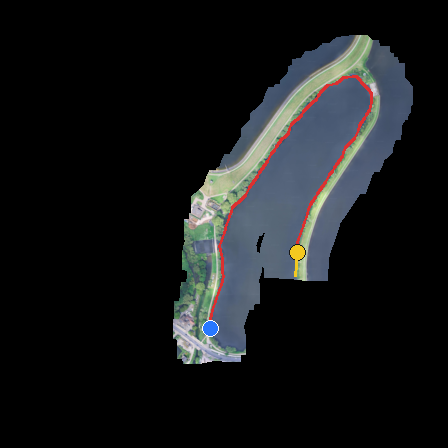
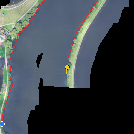
London-2: global view on the left, local view on the right. Blue marks the start, yellow marks position and heading at the window boundary, and red marks the trajectory. Images are from the paper's Map Memory appendix example.

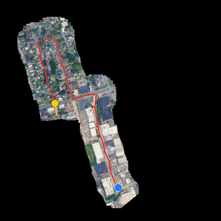
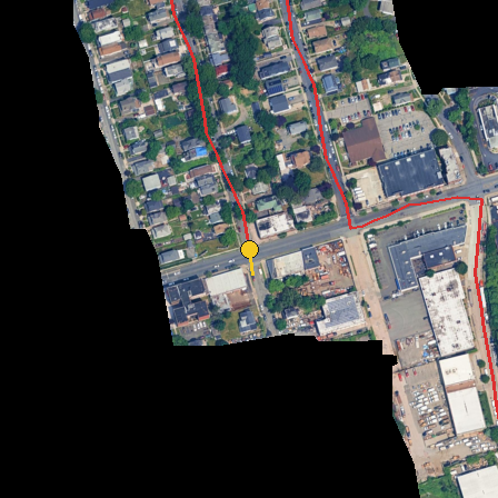
NewYork-1: global map on the left and local map on the right. Together with London-2 above, this illustrates explored coverage along different routes. Images are from the paper appendix.

A shared geographic frame brings route shape, revisited areas, and the relationship between start and current position into one image. Representation quality depends on action integration, scene imagery, and geographic alignment. The current implementation uses SatNav, which supplies these inputs.

4. How maps become memory tokens

During training, the dataset renders maps and places them in the history portion of images. During evaluation, _compute_history_cache_map() renders and encodes them. Both paths then apply per-frame compression and concatenate global-map tokens followed by local-map tokens.

The current default is COMPRESS_STRIDE=2. For Qwen2.5-VL with 448 × 448 inputs, each map produces 256 visual tokens and is further pooled to 64. Concatenating the global map followed by the local map produces a 128-token memory block.

Compression setting	Encoded tokens per map	Pooled tokens per map	Total for two maps
Default COMPRESS_STRIDE=2	\(16\times16=256\)	\(8\times8=64\)	128
COMPRESS_STRIDE=1	\(16\times16=256\)	256	512

For other image sizes or backbones, counts follow the actual image_grid_thw and merge_size. Stride controls the tradeoff between map detail and LLM context cost: a smaller stride retains a denser visual grid and more input tokens. See memory configuration for launch parameters.

5. Rendering caches and code entry points

A disk cache can reuse rendered maps for the same trajectory prefix and rendering configuration. Online inference separately keeps encoded map tokens for reuse within a window. The disk cache saves orthophoto reads and rendering; the token cache saves repeated visual encoding.

Component	Implementation
Defaults and builder composition	SatNavMapMemoryBuilder
Action integration, footprints, and image crops	MapGeometryMixin
Masks, crop centers, and trajectory drawing	MapRenderMixin
Training scene and episode metadata	metadata.py
Disk image cache	MapCacheMixin
Online encoding and pooling	_compute_history_cache_map

Paper source: SatNav paper, Memory Design Details → Map Memory. Image provenance is recorded in the asset notes.